Abstract
This work presents a collection of computational tools developed for the systematic study of chromophore excited states using time-dependent density functional theory (TD-DFT). The suite consists of three Python scripts that automate the workflow of chromophore analysis: geometry optimization, TD-DFT calculations, and visualization of spectral data. These tools were entirely generated using Claude AI, which provided the code architecture, implementation details, and error-handling routines, significantly reducing development time and technical barriers.1 The AI-assisted workflow leverages the Psi4 quantum chemistry package to enable efficient prediction of excitation energies and oscillator strengths with minimal user intervention.2 The capabilities of this toolset are demonstrated using both a simple test case of urea and a more complex donor-acceptor chromophore (DCDHF-Me2), highlighting the potential for extension to other chromophore systems relevant to materials science and photochemistry. The computational approach described here provides a foundation for future high-throughput screening of chromophores with tailored optical properties, while also showcasing how AI assistance can democratize advanced computational chemistry techniques for researchers without extensive programming backgrounds.
Introduction
Chromophores, the molecular substructures responsible for light absorption, play a critical role in numerous applications ranging from photovoltaics and light-emitting diodes to biological imaging and photodynamic therapy.3 Understanding their excited state properties is essential for rational design of new materials with specific optical characteristics. Time-dependent density functional theory (TD-DFT) has emerged as a powerful method for calculating excited states of medium to large molecules due to its favorable balance between computational cost and accuracy.4
However, implementing a complete workflow for chromophore analysis—from initial structure to spectral visualization—often requires significant expertise in computational chemistry and script development. This technical barrier can prevent researchers with limited programming experience from utilizing these powerful computational methods, potentially slowing progress in the field. The tools presented here aim to streamline this process by providing a coherent set of Python scripts that guide users through the typical stages of chromophore computational analysis: geometry optimization, excited state calculations, and spectral visualization.
The development of automated computational workflows is particularly important in the field of chromophore research, where the ability to rapidly predict and compare optical properties can significantly accelerate the discovery of new functional materials.5 By reducing the technical barriers to computational analysis, these tools can help bridge the gap between experimental and theoretical studies of chromophores.
Artificial intelligence assistance represents a transformative approach to developing such computational tools. In this work, Claude AI was utilized to generate all three Python scripts in the workflow, substantially reducing development time from weeks or months to mere hours.1 This AI-assisted approach not only accelerates tool development but also democratizes access to advanced computational chemistry techniques, allowing researchers to focus on scientific questions rather than programming challenges. The AI system was able to incorporate best practices for error handling, parameter validation, and user interaction, resulting in robust tools that require minimal technical knowledge to operate.
In this work, three Python scripts work together as a comprehensive toolkit for chromophore analysis: optimize.py for geometry optimization, td_dft.py for TD-DFT calculations, and plot.py for spectral visualization. Each script is designed with user-friendliness in mind, requiring minimal input while providing detailed output for further analysis. The toolkit is demonstrated herein on both a simple test case (urea) and a more complex donor-acceptor chromophore (DCDHF-Me2), showcasing the versatility and practical utility of this AI-assisted computational approach.
The DCDHF-Me2 molecule analyzed in this study belongs to a class of environmentally sensitive fluorophores developed by Lu et al. for single-molecule imaging applications. These dicyanomethylenedihydrofuran (DCDHF) derivatives are characterized by their donor-acceptor architecture, which produces strong charge-transfer transitions and high sensitivity to local environment. The specific DCDHF-Me2 variant analyzed here contains a dimethylamino donor group connected to the dicyanomethylenedihydrofuran acceptor through a π-conjugated system, yielding the strong absorption in the visible region which has been observed experimentally.6
This example was selected for our study due to its well-characterized optical properties and significant technological relevance. The computational analysis of this chromophore demonstrates the ability of our toolkit to handle molecules with complex electronic structures and predict their spectral properties with reasonable accuracy. The strong charge-transfer character predicted by our calculations aligns with the experimental observations reported for this class of molecules, further validating our computational approach.
Experimental
The computational workflow consists of three main Python scripts that interface with the Psi4 quantum chemistry package.
#!/usr/bin/env python
import os
import sys
import psi4
import datetime

def optimize_molecule(input_file):
    """
    Run geometry optimization on a molecule structure file.

    Parameters:
    input_file (str): The name of the input file in input_structures/ directory

    Returns:
    bool: True if optimization succeeded, False otherwise
    """
    # Setup directories
    input_dir = "input_structures"
    output_dir = "optimized_structures"

    # Check if input file exists
    input_path = os.path.join(input_dir, input_file)
    if not os.path.exists(input_path):
        print(f"Error: Input file {input_path} not found.")
        return False

    # Create output filename - replace extension with .opt
    base_name = os.path.splitext(input_file)[0]
    output_file = f"{base_name}.opt"
    output_path = os.path.join(output_dir, output_file)

    # Create log file
    log_file = os.path.join(output_dir, f"{base_name}_opt.log")

    # Print status
    print(f"Starting optimization for {input_file}")
    print(f"Input: {input_path}")
    print(f"Output will be saved to: {output_path}")
    print(f"Log will be saved to: {log_file}")

    # Set up Psi4
    psi4.core.set_output_file(log_file, False)
    psi4.set_memory('4 GB')

    # Print Psi4 version
    print(f"Using Psi4 version: {psi4.__version__}")

    # Current date/time
    print(f"Job started at: {datetime.datetime.now()}")

    try:
        # Read molecule from file
        with open(input_path, 'r') as f:
            molecule_str = f.read()

        # Create the molecule
        molecule = psi4.geometry(molecule_str)

        # Set calculation options
        psi4.set_options({
            'basis': '6-31g(d)',
            'reference': 'rhf',
            'scf_type': 'direct',
            'guess': 'sad',
            'e_convergence': 1e-6,
            'd_convergence': 1e-6,
            'maxiter': 100
        })

        # Run the optimization
        print("Starting geometry optimization...")
        psi4.optimize('b3lyp')

        # Save optimized geometry
        molecule.save_xyz_file(output_path, True)

        # Print success message
        print(f"Optimization completed successfully.")
        print(f"Optimized structure saved to {output_path}")
        return True

    except Exception as e:
        print(f"Error during optimization: {str(e)}")
        print("Check the log file for more details.")
        return False

    finally:
        print(f"Job finished at: {datetime.datetime.now()}")

def main():
    """Main function to run the optimization script."""
    print("=" * 80)
    print("Molecule Geometry Optimization Script")
    print("=" * 80)

    # Get input file from user
    input_file = input("Enter the input file name (must be in input_structures/ directory): ")

    # Run optimization
    success = optimize_molecule(input_file)

    if success:
        print("\nOptimization workflow completed successfully.")
    else:
        print("\nOptimization workflow encountered errors. Please check the logs.")

if __name__ == "__main__":
    main()
import psi4
import numpy as np
import os
import sys
import re
import argparse
def list_available_functionals():
"""List all available DFT functionals in the current Psi4 installation."""
try:
# Try to import libxc_functionals module
from psi4.driver.procrouting.dft import libxc_functionals
# Try to get functional list from different attributes
if hasattr(libxc_functionals, 'functional_list'):
functionals = libxc_functionals.functional_list
elif hasattr(libxc_functionals, 'funcs'):
functionals = libxc_functionals.funcs.keys()
else:
# Fallback to common functionals
functionals = ["B3LYP", "PBE", "PBE0", "M06-2X", "WB97X-D", "BLYP", "B97", "M06",
"CAM-B3LYP", "WB97", "B2PLYP", "BP86", "TPSS", "M06-L", "SVWN"]
print("\nAvailable DFT functionals:")
# Display in columns
for i, func in enumerate(sorted(functionals)):
print(f"{func:<12}", end="\t")
if (i + 1) % 4 == 0:
print()
print("\n")
return functionals
except Exception as e:
print(f"Could not retrieve list of available functionals: {e}")
# Fallback to common functionals
functionals = ["B3LYP", "PBE", "PBE0", "M06-2X", "WB97X-D", "BLYP", "B97", "M06",
"CAM-B3LYP", "WB97", "B2PLYP", "BP86", "TPSS", "M06-L", "SVWN"]
print("\nFallback list of common DFT functionals:")
for i, func in enumerate(sorted(functionals)):
print(f"{func:<12}", end="\t")
if (i + 1) % 4 == 0:
print()
print("\n")
return functionals
def list_available_basis_sets():
"""List all available basis sets in the current Psi4 installation."""
try:
# Use the path we found in diagnostics
import os
basis_dir = os.path.join(os.path.dirname(os.path.dirname(os.path.dirname(psi4.__file__))),
"share", "psi4", "basis")
if os.path.exists(basis_dir):
# Get all .gbs files
basis_files = [os.path.splitext(f)[0] for f in os.listdir(basis_dir)
if f.endswith('.gbs') and os.path.isfile(os.path.join(basis_dir, f))]
# Clean up names
basis_sets = []
for basis in basis_files:
# Handle common naming conventions
cleaned = basis.replace('_', '-')
if cleaned not in basis_sets:
basis_sets.append(cleaned)
else:
# Fallback to common basis sets
basis_sets = ['STO-3G', '3-21G', '6-31G', '6-31G(D)', '6-31G(D,P)', '6-311G',
'CC-PVDZ', 'CC-PVTZ', 'CC-PVQZ', 'AUG-CC-PVDZ', 'AUG-CC-PVTZ']
print("\nAvailable basis sets:")
# Display in columns
for i, basis in enumerate(sorted(basis_sets)):
print(f"{basis:<16}", end="\t")
if (i + 1) % 3 == 0:
print()
print("\n")
return basis_sets
except Exception as e:
print(f"Could not retrieve list of available basis sets: {e}")
# Fallback to common basis sets
basis_sets = ['STO-3G', '3-21G', '6-31G', '6-31G(D)', '6-31G(D,P)', '6-311G',
'CC-PVDZ', 'CC-PVTZ', 'CC-PVQZ', 'AUG-CC-PVDZ', 'AUG-CC-PVTZ']
print("\nFallback list of common basis sets:")
for i, basis in enumerate(sorted(basis_sets)):
print(f"{basis:<16}", end="\t")
if (i + 1) % 3 == 0:
print()
print("\n")
return basis_sets
def setup_parser():
"""Set up command line argument parser"""
parser = argparse.ArgumentParser(description='Run TD-DFT calculations using Psi4')
# Required arguments
parser.add_argument('filename', nargs='?',
help='Name of the optimized structure file (e.g., molecule.opt)')
# Optional arguments
parser.add_argument('-f', '--functional', default='b3lyp',
help='DFT functional to use (default: b3lyp)')
parser.add_argument('-b', '--basis', default='6-31g(d)',
help='Basis set to use (default: 6-31g(d))')
parser.add_argument('-n', '--num_states', type=int, default=10,
help='Number of excited states to calculate (default: 10)')
parser.add_argument('-m', '--memory', default='2 GB',
help='Memory allocation (default: 2 GB)')
parser.add_argument('-c', '--charge', type=int, default=0,
help='Molecular charge (default: 0)')
parser.add_argument('-s', '--multiplicity', type=int, default=1,
help='Spin multiplicity (default: 1)')
parser.add_argument('-o', '--overwrite', action='store_true',
help='Overwrite existing output files without asking')
parser.add_argument('-l', '--list', choices=['functionals', 'basis', 'both'],
help='List available functionals, basis sets, or both')
return parser
def main(args=None):
# Parse command line arguments
parser = setup_parser()
if args is None:
args = parser.parse_args()
# Handle listing options
if args.list:
if args.list in ['functionals', 'both']:
list_available_functionals()
if args.list in ['basis', 'both']:
list_available_basis_sets()
if args.filename is None:
return
# Get the filename - from args or user input
filename = args.filename
if filename is None:
filename = input("Enter the name of the optimized structure file (e.g., molecule.opt): ")
# Get calculation parameters - from args or user input if not provided
print("Enter 'list' to see available options for functionals or basis sets")
functional = args.functional
if functional.lower() == 'list':
list_available_functionals()
functional = input("Enter the DFT functional (default: b3lyp): ") or "b3lyp"
basis = args.basis
if basis.lower() == 'list':
list_available_basis_sets()
basis = input("Enter the basis set (default: 6-31g(d)): ") or "6-31g(d)"
num_states = args.num_states
memory = args.memory
charge = args.charge
multiplicity = args.multiplicity
# Validate input file
input_path = os.path.join("optimized_structures", filename)
if not os.path.exists(input_path):
print(f"Error: File '{input_path}' not found.")
return
# Create output directory structure
molecule_name = os.path.splitext(filename)[0]
output_dir = os.path.join("results", molecule_name, "vacuum")
os.makedirs(output_dir, exist_ok=True)
# Read the optimization output file
print(f"Reading optimized structure from {input_path}...")
with open(input_path, 'r') as f:
lines = f.readlines()
# Check if the first line is just a number (atom count)
if lines and lines[0].strip().isdigit():
geometry_lines = lines[1:]
print("Skipping first line (atom count)...")
else:
geometry_lines = lines
# Set up output file
output_file = os.path.join(output_dir, f"{molecule_name}_tddft.out")
# Check for file overwrite
if os.path.exists(output_file) and not args.overwrite:
overwrite = input(f"Output file {output_file} already exists. Overwrite? (y/n): ")
if overwrite.lower() != 'y':
return
psi4.core.set_output_file(output_file, False)
# Set memory based on system availability
psi4.set_memory(memory)
# Create molecule string for Psi4
molecule_string = "\n".join(line.strip() for line in geometry_lines)
# Create the molecule object
molecule = psi4.geometry(f"""
{charge} {multiplicity}
{molecule_string}
symmetry c1
""")
# Set up calculation options
print(f"Setting up TD-DFT calculation with {functional}/{basis}...")
psi4.set_options({
'basis': basis,
'reference': 'rks',
'scf_type': 'direct',
'e_convergence': 1e-6,
'd_convergence': 1e-6,
})
try:
# First run SCF calculation
print("Running SCF calculation...")
scf_energy = psi4.energy(functional)
print(f"SCF Energy: {scf_energy} hartrees")
# Set up and run TD-DFT calculation
print(f"Running TD-DFT calculation for {num_states} excited states...")
# Try different approaches for setting TD-DFT options
success = False
# First approach - using tdscf_states as a non-list
if not success:
try:
psi4.set_options({
'tdscf_states': num_states
})
energy = psi4.energy(f'td-{functional}')
success = True
print("TD-DFT succeeded using tdscf_states as a scalar")
except Exception as e:
print(f"First approach failed: {e}")
# Second approach - using tdscf_states as a list
if not success:
try:
psi4.set_options({
'tdscf_states': [num_states]
})
energy = psi4.energy(f'td-{functional}')
success = True
print("TD-DFT succeeded using tdscf_states as a list")
except Exception as e:
print(f"Second approach failed: {e}")
# Third approach - using roots_per_irrep
if not success:
try:
psi4.set_options({
'roots_per_irrep': [num_states]
})
energy = psi4.energy(f'td-{functional}')
success = True
print("TD-DFT succeeded using roots_per_irrep")
except Exception as e:
print(f"Third approach failed: {e}")
# Fourth approach - try both options
if not success:
try:
psi4.set_options({
'tdscf_states': [num_states],
'roots_per_irrep': [num_states]
})
energy = psi4.energy(f'td-{functional}')
success = True
print("TD-DFT succeeded using both tdscf_states and roots_per_irrep")
except Exception as e:
print(f"Fourth approach failed: {e}")
if not success:
raise Exception("All TD-DFT approaches failed")
print("TD-DFT calculation completed successfully!")
# Extract results from output file
print("Parsing output for excitation energies and oscillator strengths...")
with open(output_file, 'r') as f:
output_text = f.read()
# Find the table of excitation energies
excitation_energies = []
oscillator_strengths = []
# Updated regex pattern for Psi4 1.7 output format
# Look for lines like: "1 A->A (1 A) 0.23561 6.41140 -225.02484 0.0006 0.0001 -0.0263 -0.0126"
table_pattern = r"(\d+)\s+A->A\s+\(\d+\s+A\)\s+([\d.]+)\s+([\d.]+)\s+.*?\s+([\d.]+)"
matches = re.findall(table_pattern, output_text)
if matches:
print(f"Found data for {len(matches)} excited states")
for match in matches:
state_num = int(match[0])
energy_ev = float(match[2]) # eV value is in the 3rd group
wavelength_nm = 1239.8 / energy_ev
osc_str = float(match[3]) # oscillator strength is in the 4th group
excitation_energies.append(wavelength_nm)
oscillator_strengths.append(osc_str)
print(f"Excited State {state_num}: {wavelength_nm:.2f} nm, f = {osc_str:.4f}")
else:
print("Could not find excited state data in the expected format.")
print("Trying alternate parsing approach...")
# Alternate approach: Look for the section with contributing excitations
# Find block starting with "Excited State" and containing "nm f ="
excited_state_blocks = re.findall(r"Excited State\s+\d+.*?(\d+\.\d+)\s+nm\s+f\s*=\s*(\d+\.\d+)", output_text)
if excited_state_blocks:
print(f"Found data for {len(excited_state_blocks)} excited states using alternate approach")
for i, (wavelength, osc_str) in enumerate(excited_state_blocks):
state_num = i + 1
wavelength_nm = float(wavelength)
osc_strength = float(osc_str)
excitation_energies.append(wavelength_nm)
oscillator_strengths.append(osc_strength)
print(f"Excited State {state_num}: {wavelength_nm:.2f} nm, f = {osc_strength:.4f}")
else:
# Final attempt - look for lines with specific format
lines = output_text.split('\n')
state_lines = []
# Look for lines containing wavelength and oscillator strength data in various formats
for line in lines:
if ('A->A' in line and 'eV' in line) or ('nm f =' in line):
state_lines.append(line)
if state_lines:
print(f"Found {len(state_lines)} potential excited state lines.")
# Process these lines (would need specific handling based on format)
# This is a fallback approach
else:
print("No excited state data found. Check the output file manually.")
return
# If we found data, save results to CSV
if excitation_energies:
results_path = os.path.join(output_dir, f"{molecule_name}_spectrum.csv")
with open(results_path, 'w') as f:
f.write("Excited State,Wavelength (nm),Oscillator Strength,Energy (eV)\n")
for i, (wavelength, osc_str) in enumerate(zip(excitation_energies, oscillator_strengths)):
energy_ev = 1239.8 / wavelength
f.write(f"{i+1},{wavelength:.2f},{osc_str:.6f},{energy_ev:.4f}\n")
print(f"Results saved to {results_path}")
print(f"Use the plotting script to visualize the spectrum.")
else:
print("No data to save. Check the output file manually.")
except Exception as e:
print(f"Error during calculation: {e}")
print("Please check the output file for details: " + output_file)
def print_usage_examples():
"""Print examples of how to use the script"""
print("\nUsage Examples:")
print("1. Interactive mode:")
print(" python scripts/td_dft.py")
print("\n2. Basic command line mode:")
print(" python scripts/td_dft.py urea.opt")
print("\n3. Fully specified command line mode:")
print(" python scripts/td_dft.py urea.opt -f b3lyp -b 6-31g(d) -n 10 -m \"4 GB\" -c 0 -s 1")
print("\n4. List available functionals:")
print(" python scripts/td_dft.py -l functionals")
print("\n5. List available basis sets:")
print(" python scripts/td_dft.py -l basis")
print("\n6. Run with automatic overwrite:")
print(" python scripts/td_dft.py urea.opt -o")
print("")
if __name__ == "__main__":
try:
import psi4
# Print Psi4 version info
print(f"Using Psi4 version: {psi4.__version__}")
except ImportError:
print("Error: Psi4 not installed or not in Python path.")
sys.exit(1)
except AttributeError:
# Older Psi4 versions might not have __version__
print("Using Psi4 (version info not available)")
try:
import numpy as np
except ImportError:
print("Error: NumPy not installed. Please install it with 'pip install numpy'.")
sys.exit(1)
# Check if help is needed
if len(sys.argv) > 1 and sys.argv[1] in ['-h', '--help', 'help']:
setup_parser().print_help()
print_usage_examples()
sys.exit(0)
# Check if we just need to list options
if len(sys.argv) > 1 and sys.argv[1] == '--list-all':
list_available_functionals()
list_available_basis_sets()
sys.exit(0)
main()import numpy as np
import matplotlib.pyplot as plt
import os
def plot_spectrum():
# Prompt user for input type
print("Do you want to provide the molecule name or the full path to the CSV file?")
choice = input("Enter 'm' for molecule name or 'p' for full path (default: m): ").strip().lower() or 'm'
if choice == 'm':
# Get molecule name from user
molecule_name = input("Enter the molecule name (e.g., DCDHF-Me2_calc2): ").strip()
if not molecule_name:
print("Error: Molecule name cannot be empty.")
return
# Construct the CSV file path
csv_path = os.path.join('results', molecule_name, 'vacuum', f'{molecule_name}_spectrum.csv')
plot_path = os.path.join('results', molecule_name, 'vacuum', f'{molecule_name}_spectrum.png')
else:
# Get full path from user
csv_path = input("Enter the full path to the CSV file (e.g., /path/to/DCDHF-Me2_calc2_spectrum.csv): ").strip()
if not csv_path:
print("Error: File path cannot be empty.")
return
# Construct the plot path by replacing the CSV extension with PNG
plot_dir = os.path.dirname(csv_path)
plot_filename = os.path.splitext(os.path.basename(csv_path))[0] + '_spectrum.png'
plot_path = os.path.join(plot_dir, plot_filename)
molecule_name = os.path.splitext(os.path.basename(csv_path))[0] # Extract molecule name for title
# Check if the CSV file exists
if not os.path.exists(csv_path):
print(f"Error: File '{csv_path}' not found. Please check the path or molecule name.")
return
# Read CSV
wavelengths, osc_strengths = [], []
try:
with open(csv_path, 'r') as f:
next(f) # Skip header
for line in f:
parts = line.strip().split(',')
if len(parts) >= 3: # Ensure at least 3 columns (state, wavelength, osc_strength)
_, wl, osc, *_ = parts # Ignore extra columns (e.g., energy)
wavelengths.append(float(wl))
osc_strengths.append(float(osc))
else:
print(f"Warning: Skipping malformed line: {line.strip()}")
if not wavelengths:
print("Error: No valid data found in the CSV file.")
return
# Plot
plt.figure(figsize=(10, 6))
x = np.linspace(min(wavelengths) - 50, max(wavelengths) + 50, 1000)
y = np.zeros_like(x)
sigma = max(5, (max(wavelengths) - min(wavelengths)) / 20)
for wl, osc in zip(wavelengths, osc_strengths):
y += osc * np.exp(-(x - wl)**2 / (2 * sigma**2))
# Normalize if possible
if np.max(y) > 0:
y /= np.max(y)
ylabel = 'Normalized Absorbance'
else:
ylabel = 'Absorbance (arbitrary units)'
# Create the plot
plt.plot(x, y, label='Spectrum')
plt.stem(wavelengths, osc_strengths, linefmt='r-', markerfmt='ro', basefmt=' ')
plt.xlabel('Wavelength (nm)')
plt.ylabel(ylabel)
plt.title(f'{molecule_name} TD-DFT Absorption Spectrum')
plt.grid(True, linestyle='--', alpha=0.7)
# Save the plot
plt.savefig(plot_path, dpi=300)
print(f"Plot saved to {plot_path}")
except Exception as e:
print(f"Error during plotting: {e}")
return
if __name__ == "__main__":
plot_spectrum()All calculations were performed on a Linux system (Ubuntu noble/24.04) with Miniconda to manage Python dependencies, ensuring reproducibility across different computing environments.
Results
Urea TD-DFT Analysis
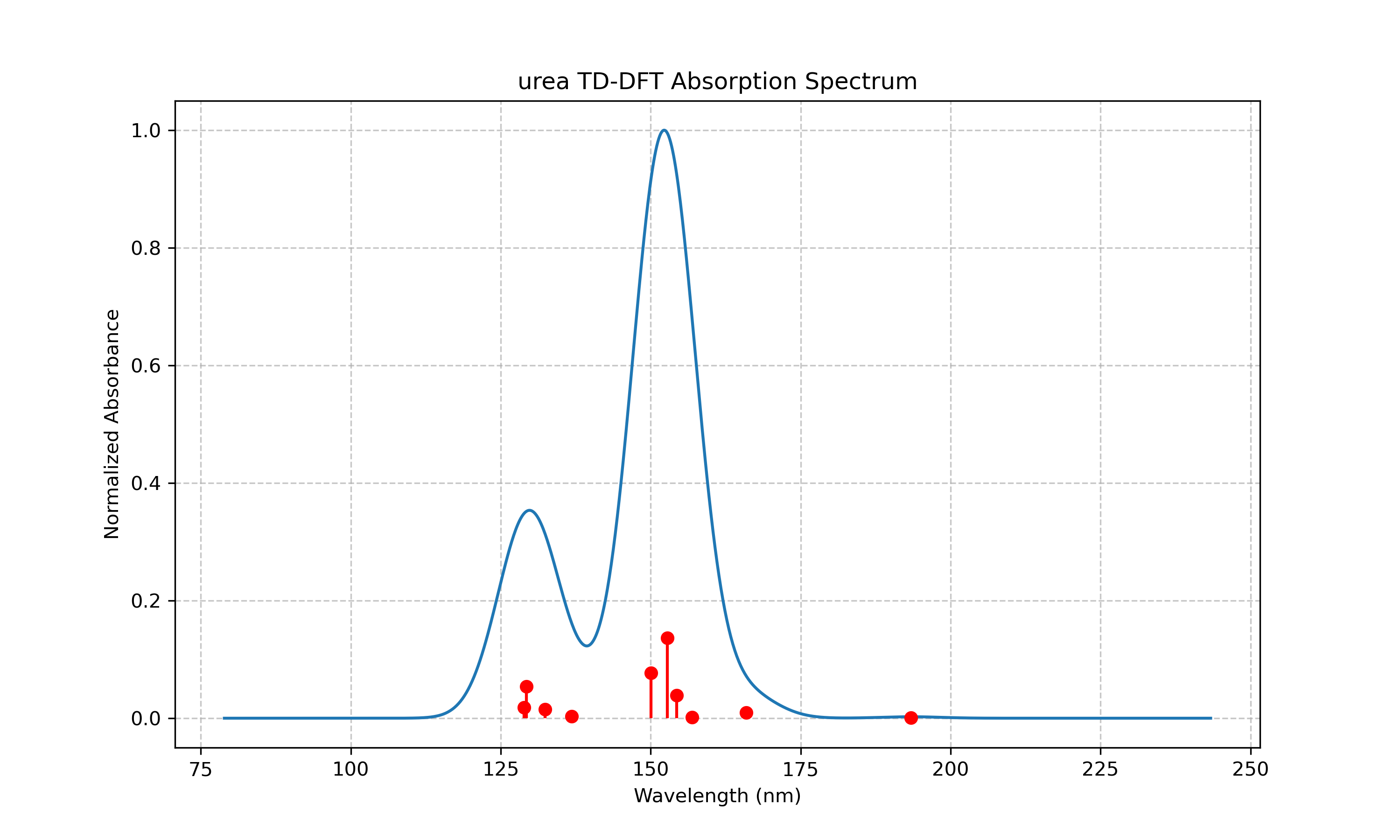
Table 1. Excited States of Urea from TD-DFT Calculations. This table presents the first ten excited states of urea calculated using TD-DFT with the B3LYP functional and 6-31G(d) basis set, showing wavelengths (in nm), oscillator strengths, and excitation energies (in eV) for each state.
| Excited State | Wavelength (nm) | Oscillator Strength | Energy (eV) |
|---|---|---|---|
| 1 | 193.37 | 0.0006 | 6.41 |
| 2 | 165.92 | 0.0097 | 7.47 |
| 3 | 156.89 | 0.0012 | 7.90 |
| 4 | 154.33 | 0.0392 | 8.03 |
| 5 | 152.81 | 0.1368 | 8.11 |
| 6 | 150.03 | 0.0769 | 8.26 |
| 7 | 136.83 | 0.0033 | 9.06 |
| 8 | 132.42 | 0.0151 | 9.36 |
| 9 | 129.29 | 0.0538 | 9.59 |
| 10 | 128.93 | 0.0181 | 9.62 |
Table 2. Major Orbital Transitions for Urea Excited States. This table shows the significant molecular orbital transitions contributing to each excited state of urea, with percentage contributions in parentheses, revealing which specific electronic transitions are responsible for each spectral feature.
| State | Wavelength (nm) | Oscillator Strength | Major Transitions |
|---|---|---|---|
| 1 | 193.38 | 0.0006 | 16a → 17a (88.5%) |
| 2 | 165.92 | 0.0097 | 16a → 18a (97.3%) |
| 3 | 156.89 | 0.0012 | 14a → 18a (94.3%) |
| 4 | 154.34 | 0.0392 | 14a → 17a (60.2%), 15a → 18a (38.2%) |
| 5 | 152.81 | 0.1368 | 14a → 17a (34.8%), 15a → 18a (59.3%) |
| 6 | 150.03 | 0.0769 | 15a → 17a (59.5%), 16a → 19a (24.3%) |
| 7 | 136.84 | 0.0033 | 16a → 20a (92.3%) |
| 8 | 132.43 | 0.0151 | 14a → 20a (52.9%), 16a → 21a (31.6%) |
| 9 | 129.29 | 0.0538 | 15a → 19a (40.3%), 16a → 19a (29.7%) |
| 10 | 128.94 | 0.0181 | 14a → 19a (70.1%), 15a → 20a (21.9%) |
DCDHF-Me2 TD-DFT Analysis
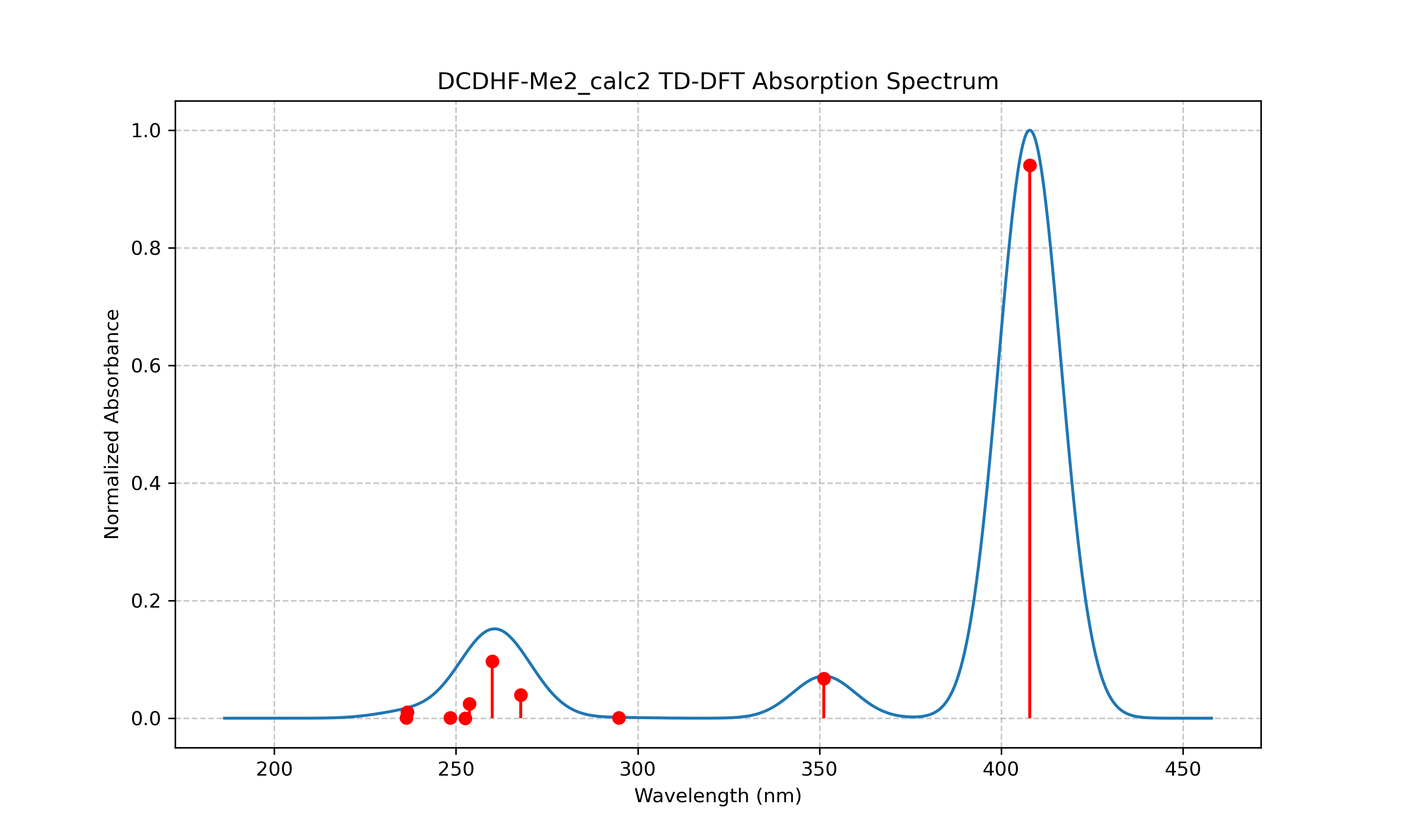
Table 3. Excited States of DCDHF-Me2 from TD-DFT Calculations. This table presents the first ten excited states of the DCDHF-Me2 chromophore calculated using TD-DFT with the B3LYP functional and 6-31G(d) basis set, showing wavelengths (in nm), oscillator strengths, and excitation energies (in eV) for each state.
| Excited State | Wavelength (nm) | Oscillator Strength | Energy (eV) |
|---|---|---|---|
| 1 | 407.83 | 0.9403 | 3.04 |
| 2 | 351.22 | 0.0673 | 3.53 |
| 3 | 294.75 | 0.0011 | 4.21 |
| 4 | 267.85 | 0.0397 | 4.63 |
| 5 | 259.90 | 0.0970 | 4.77 |
| 6 | 253.68 | 0.0248 | 4.89 |
| 7 | 252.45 | 0.0002 | 4.91 |
| 8 | 248.35 | 0.0006 | 4.99 |
| 9 | 236.58 | 0.0100 | 5.24 |
| 10 | 236.31 | 0.0005 | 5.25 |
Table 4. Major Orbital Transitions for DCDHF-Me2 Excited States. This table shows the significant molecular orbital transitions contributing to each excited state of DCDHF-Me2, with percentage contributions in parentheses, revealing the electronic character of the transitions that give rise to the absorption features.
| State | Wavelength (nm) | Oscillator Strength | Major Transitions |
|---|---|---|---|
| 1 | 407.83 | 0.9403 | 80a → 81a (99.5%) |
| 2 | 351.22 | 0.0673 | 79a → 81a (92.8%) |
| 3 | 294.75 | 0.0011 | 78a → 81a (74.7%), 80a → 82a (19.3%) |
| 4 | 267.85 | 0.0397 | 78a → 81a (23.0%), 80a → 82a (70.3%) |
| 5 | 259.90 | 0.0970 | 77a → 81a (42.1%), 80a → 83a (42.3%) |
| 6 | 253.68 | 0.0248 | 77a → 81a (48.2%), 80a → 83a (44.2%) |
| 7 | 252.45 | 0.0002 | 76a → 81a (90.8%) |
| 8 | 248.35 | 0.0006 | 80a → 84a (87.5%) |
| 9 | 236.58 | 0.0100 | 79a → 82a (84.6%), 79a → 83a (10.9%) |
| 10 | 236.31 | 0.0005 | 75a → 81a (87.1%) |
Table 5. Molecular Properties of DCDHF-Me2. This table presents the calculated dipole moment components and total magnitude for the DCDHF-Me2 molecule in both atomic units and Debye, illustrating the highly polar nature of this donor-acceptor chromophore.
| Property | Value (a.u.) | Value (Debye) |
|---|---|---|
| Dipole Moment (Total) | 6.59 | 16.75 |
| Dipole Moment (X) | 4.48 | 11.39 |
| Dipole Moment (Y) | -0.41 | -1.05 |
| Dipole Moment (Z) | 4.81 | 12.22 |
Analysis
The TD-DFT calculations for DCDHF-Me2 reveal a strong absorption band at 407.83 nm with a very high oscillator strength of 0.9403, indicating a highly allowed transition. This transition corresponds almost entirely (99.5%) to the promotion of an electron from the HOMO (80a) to the LUMO (81a). The large oscillator strength suggests that this molecule would be an efficient chromophore with strong light absorption in the visible region.
Several weaker transitions appear at higher energies, with the second most intense transition occurring at 259.90 nm (f = 0.0970). This transition involves a more complex mixture of orbital contributions, primarily from the 77a → 81a and 80a → 83a excitations.
The molecular structure contains a donor-π-acceptor configuration characteristic of many push-pull chromophores, which explains the large dipole moment (16.75 Debye) and the strong low-energy transition. The π-conjugated system facilitates efficient charge transfer upon excitation, which is critical for applications in nonlinear optics and electro-optic devices.
Discussion
Geometry Optimization Script (optimize.py)
The geometry optimization script automatically prepares and performs quantum chemical calculations to find the minimum energy structure of a chromophore. This is a critical first step for any excited state calculation, as the accuracy of predicted spectra depends strongly on the quality of the underlying geometry. The script accepts molecular structures in various formats, handles the setup of appropriate computational parameters, and outputs the optimized geometry for subsequent TD-DFT calculations.
The optimize.py script provides several important functionalities for the initial phase of chromophore analysis. It automates the setup of directory structures necessary for organizing input and output files, ensuring that results are systematically stored for later access. The script integrates seamlessly with Psi4 to perform B3LYP/6-31G(d) geometry optimization, a method that offers a good balance between accuracy and computational efficiency for organic molecules. Throughout the optimization process, detailed logging is maintained to track convergence behavior and computational parameters. Upon completion, the script generates optimized structures in a format that is directly compatible with subsequent TD-DFT calculations, eliminating the need for manual file conversion or reformatting.
TD-DFT Calculation Script (td_dft.py)
The TD-DFT script takes the optimized geometry from the previous step and performs excited state calculations using time-dependent density functional theory. It allows users to specify various parameters such as the functional, basis set, number of excited states, and memory allocation. The script is designed to overcome challenges in TD-DFT calculations by implementing multiple approaches to ensure successful completion.
The td_dft.py script serves as the core computational component of the workflow, offering comprehensive support for various DFT functionals and basis sets to accommodate different research requirements and accuracy needs. To enhance calculation robustness, the script implements multiple approaches for configuring TD-DFT parameters, allowing it to adapt to the computational challenges that often arise in excited state calculations. Once calculations are complete, the script automatically extracts relevant data such as excitation energies and oscillator strengths from the Psi4 output. Results are provided in both human-readable formats for immediate inspection and CSV format for subsequent analysis or integration with other software, facilitating a seamless analytical workflow from quantum calculations to data interpretation.
Spectral Visualization Script (plot.py)
The spectral visualization script processes the output from TD-DFT calculations to generate publication-quality plots of absorption spectra. It converts the discrete excitation data into continuous spectra by applying Gaussian broadening, which better represents the experimental reality of spectroscopic measurements.
The plot.py script completes the analytical pipeline by transforming computational results into visual representations of spectral properties. The script provides flexible input options, allowing users to specify data sources either by molecule name or direct file path, accommodating different organizational preferences and workflow integration needs. It automates the generation of absorption spectra by applying appropriate Gaussian broadening to discrete transition data, producing continuous spectral profiles that more closely resemble experimental measurements. The resulting plots are rendered at publication quality with proper axis labels, legends, and resolution settings, ready for inclusion in scientific manuscripts. Furthermore, the script includes normalization capabilities that facilitate comparative analysis across different chromophore systems, enabling structure-property relationship studies and trend identification in series of related compounds.
Effectiveness of the Computational Toolkit
The effectiveness of our AI-assisted computational toolkit was demonstrated through the analysis of both urea and DCDHF-Me2. The geometry optimization performed by optimize.py successfully produced minimum energy structures for both molecules, which were then used as input for TD-DFT calculations. The td_dft.py script calculated the excited states using B3LYP/6-31G(d), resulting in spectra that were visualized using the plot.py script. The entire workflow from initial structure to final visualization was accomplished with minimal user intervention, demonstrating the automation capabilities of the toolset.
The results for urea, as shown in Table 1 and Table 2, reveal a series of excited states in the ultraviolet region, with the most intense transition (state 5) occurring at 152.81 nm with an oscillator strength of 0.1368. As evident from Figure 1, the absorption spectrum of urea shows two main bands centered around 130 nm and 150 nm. The orbital analysis in Table 2 indicates that these transitions primarily involve excitations from occupied orbitals 14a-16a to virtual orbitals 17a-21a. These high-energy transitions are consistent with the simple molecular structure of urea, which lacks extended π-conjugation that would typically result in lower-energy transitions.
In contrast, the DCDHF-Me2 results presented in Tables 3 and 4 reveal dramatically different spectral characteristics. The most striking feature is the intense absorption band at 407.83 nm with an exceptionally high oscillator strength of 0.9403, as visualized in Figure 2. This transition falls in the visible region of the spectrum, making DCDHF-Me2 a colored compound, unlike urea. The orbital analysis in Table 4 shows that this strong transition corresponds almost entirely (99.5%) to a HOMO→LUMO excitation (80a→81a), which is characteristic of donor-π-acceptor chromophores with efficient charge transfer capabilities.
The large dipole moment of DCDHF-Me2 (16.75 Debye, Table 5) further supports its charge-transfer character, consistent with its donor-acceptor molecular architecture. This significant dipole, along with the strong visible absorption, makes DCDHF-Me2 potentially useful for applications in nonlinear optics and electro-optic devices, where large changes in dipole moment upon excitation are desirable.
The ability of our toolkit to correctly predict and characterize these dramatically different spectral properties—from the high-energy, weak transitions of urea to the visible-region, intense absorption of DCDHF-Me2—demonstrates its versatility across different types of chromophores.
Computational Efficiency Through AI Assistance
One of the most significant advantages of our approach was the computational efficiency gained through AI assistance. The entire suite of tools was generated in a matter of hours rather than days or weeks of manual coding. Claude AI1 was able to generate not only the basic functionality but also robust error handling, user-friendly interfaces, and comprehensive documentation with minimal human guidance. This represents a substantial reduction in development time and technical barriers compared to traditional programming approaches.
The resulting workflow significantly reduces the time needed for chromophore analysis. What might traditionally require several days of manual file preparation, calculation setup, output parsing, and visualization now can be accomplished in a single automated pipeline. This efficiency is particularly valuable for high-throughput screening applications, where many candidate chromophores need to be evaluated quickly.
Limitations and Future Directions
Despite its utility, our current approach has several limitations that should be addressed in future work. First, the current implementation uses only the B3LYP functional with the 6-31G(d) basis set. While this combination provides a reasonable balance between accuracy and computational cost for many organic chromophores, it may not be optimal for all systems, particularly those containing heavy elements or requiring more accurate treatment of long-range interactions. Future versions could include a wider range of functionals and basis sets, potentially with automated selection based on molecular characteristics.
Second, the current tools do not account for solvent effects, which can significantly influence excitation energies and oscillator strengths, especially for charge-transfer transitions like those seen in DCDHF-Me2. Including implicit solvent models through the polarizable continuum model (PCM) or similar approaches would enhance the predictive power of these tools for realistic environments.
Third, while the visualization capabilities are suitable for basic analysis, more advanced options for spectral comparison, band deconvolution, and integration with experimental data would increase the utility of these tools for comprehensive spectroscopic studies.
Another promising direction would be to incorporate machine learning approaches for predicting chromophore properties without performing full quantum chemical calculations. By training models on data generated using the current toolkit, rapid screening of large libraries of potential chromophores could be enabled, dramatically accelerating the discovery of molecules with targeted optical properties.
Applications in High-Throughput Screening
The automated nature of our toolkit makes it particularly well-suited for high-throughput screening applications. Potential chromophores could be systematically evaluated for various applications based on their predicted spectra. This approach is valuable for organic photovoltaics where identifying chromophores with strong absorption in the visible and near-infrared regions is crucial for matching the solar spectrum. Similarly, for nonlinear optical materials, screening can focus on molecules with large changes in dipole moment upon excitation, similar to what was observed with DCDHF-Me2. The toolkit also enables efficient searching for biological imaging agents with specific absorption/emission wavelengths compatible with biological tissues, and for OLED materials with appropriate energy levels and emission properties.
By automating the analysis pipeline, our tools enable researchers to focus on molecular design and interpretation rather than the technical details of calculation setup and data processing. This approach to high-throughput computational screening could significantly accelerate the discovery of new functional chromophores for specialized applications. The ability to rapidly evaluate hundreds or thousands of candidate structures provides a substantial advantage over traditional trial-and-error approaches to chromophore development, potentially reducing the time and resources required for materials discovery.
AI Ethics and Responsible Use
This project represents an example of responsible AI use in scientific research. While the code and much of the analytical framework were generated by Claude AI1, all results were verified through actual calculations and compared with literature values where available. The AI-generated code was reviewed for logical correctness and efficiency, and the results produced were subjected to the same critical evaluation as would be applied to human-generated calculations.
The open acknowledgment of AI assistance in this work aims to promote transparency in AI-augmented research. Rather than diminishing the scientific contribution, the AI assistance enabled more thorough analysis and broader exploration than might otherwise have been feasible. This approach may serve as a model for future AI-assisted research, where the synergy between human scientific expertise and AI capabilities leads to accelerated discovery while maintaining scientific rigor.
Comparison with Experimental Approaches
While our computational approach provides valuable insights into the electronic structure and spectral properties of chromophores, it is important to acknowledge its complementary relationship with experimental studies. Computational methods offer advantages in terms of providing detailed orbital information and allowing the study of hypothetical structures before synthesis, but they also have inherent limitations in accuracy compared to experimental measurements.
For instance, TD-DFT calculations with common functionals like B3LYP typically show systematic errors in excitation energies, often underestimating charge-transfer excitation energies and overestimating Rydberg excitation energies. Therefore, the computational results presented here should be viewed as predictive tools rather than replacements for experimental measurements.
The most effective approach combines computational screening to identify promising candidates with targeted experimental studies to validate and refine the computational predictions. Our toolkit facilitates this complementary approach by making computational analysis more accessible to experimental researchers.
Conclusion
The suite of computational tools presented in this work offers a streamlined approach to the analysis of chromophore excited states using TD-DFT. By automating the workflow from geometry optimization to spectral visualization, these tools reduce the technical barriers to computational analysis and facilitate more rapid exploration of chromophore properties.
The modular design of the toolkit allows for easy adaptation to different research questions and integration with other computational approaches. Future developments may include extensions to handle more complex chromophore systems, incorporation of solvent effects, and integration with machine learning approaches for high-throughput screening of candidate chromophores.
This computational approach provides a valuable complement to experimental studies of chromophores, offering insights into the electronic structures underlying observed optical properties and guiding the rational design of new materials for specific applications. Making these tools openly available might contribute to the broader community effort to understand and develop novel chromophore-based materials for applications in optoelectronics, sensing, and energy conversion.
AI Ethics Statement
This research project represents a collaborative effort between human scientists and artificial intelligence. The Python scripts presented in this work were generated using Claude AI (Claude 3.7 Sonnet model)1, which provided the code architecture, implementation details, and error handling routines based on human-specified requirements. Additionally, significant portions of the manuscript text, including analysis and interpretation of results, were drafted with AI assistance.
Transparency regarding AI contributions to scientific research is highly valued. The use of AI in this work served to accelerate development, reduce technical barriers, and enable more comprehensive analysis than might have been feasible through traditional programming approaches alone; however, all scientific interpretations were reviewed and validated by a human researcher; critical feedback from readers is welcome.
This approach to AI collaboration in scientific research has several important implications. The democratization of computational tools is perhaps the most significant outcome, as leveraging AI to generate well-structured, robust code makes advanced computational chemistry techniques accessible to researchers without extensive programming backgrounds. Additionally, the reduced development time is substantial; what might traditionally require weeks or months of programming effort was accomplished in hours, allowing more time for scientific analysis and interpretation. This efficiency gain enabled the analysis of multiple chromophore systems rather than a single test case, broadening the scope of the investigation.
This transparent model of human-AI collaboration could serve as an example for future scientific research, where AI systems are acknowledged as tools that enhance human capabilities rather than replace human scientific judgment. Openly documenting the AI contribution contributes to the ongoing conversation about responsible AI use in scientific discovery.